Master industrial automation with our akYtec ALP Lesson 1. Learn to install ALP software, navigate the FBD interface, and validate logic via offline simulation. A professional bridge for hobbyists moving into B2B PLC programming and industrial control systems.
🎯 The Goal
The primary objective of this lesson is to transition from line-based coding (C++/Arduino) to visual logic design (Function Block Diagram). You will establish a professional development environment and validate your first industrial “latching” circuit without needing physical hardware.
🏆 Course Outcome: What You Will Achieve
By the end of this full akYtec series, you will have moved from a “maker” mindset to an Industrial Integrator mindset. You will be able to:
- Design professional-grade logic layouts tailored for the PR200 series programmable relays.
- Interface physical sensors, switches, and transducers directly with standard 24V DC or 230V AC industrial control voltages.
- Program onboard HMI display screens on the PR200 to visualize real-time runtime parameters and machine data.
- Implement Modbus Communication protocols to seamlessly link your physical akYtec deployments with Node-RED automation systems.
- Deploy a fully validated, 24/7 reliable control panel completely suitable for deployment in small-scale industrial B2B environments.
🛠️ Step 1: Downloading & Verifying akYtec ALP
Unlike Arduino, which relies on text-based C++, akYtec environments utilize ALP (akYtec Logic Programming). This software package is strictly based on the visual IEC 61131-3 standard using a Function Block Diagram (FBD) editor. This course was constructed and validated using akYtec ALP Version 2.11.
- Navigate directly to the official akYtec Download Center.
- Locate and download the free installer package for akYtec ALP. The software is completely open—requiring zero subscription fees, hardware key dongles, or licensing contracts, which makes it an ideal B2B entry point for small integration shops.
🔒 Professional Best Practice (Scan Before Execution)
Before launching any specialized vendor executable or driver on an active engineering workstation, you should always verify file integrity. Take your downloaded installer package and scan its signature fingerprint. You can follow our detailed guide on Why VirusTotal is the First Line of Defense for Industrial Systems to cross-check the binary across multi-engine security layers before deployment.
💻 Step 2: Installation, Target Selection & First Launch
- Extract the downloaded configuration setup file along with its companion reference manuals into your preferred local workspace directory.
- Execute the
.exeinstaller wizard. Select your preferred system operating language during this prompt (note that you can also reconfigure this setting later from the inner software options panel). - Launch the application and select “Create New Project” from the landing dashboard.
- Device Hardware Configuration: Scroll down the target hardware list and locate the PR200 series. The system lists both 230V AC and 24V DC nominal power supply device variants. For this practical course, explicitly select the PR200-24.1.X variant.
The PR200-24.1.X is a highly modular, industrial programmable relay equipped with a built-in two-line LCD display screen. Based on the manufacturer hardware definitions verified in our selection profile, this target device configuration includes the following characteristics:
- Physical UI Interface: Monochrome graphic display screen providing 16 characters alongside full multi-language formatting support, 6 custom programmable navigation buttons, and 2 independently adjustable status LEDs.
- Control Voltage Power Profile: Built-in 24V DC power supply for analog sensors and control (available only on 230V models).
- I/O Distribution Metrics: Out-of-the-box configuration featuring 8 Digital Inputs, 6 Digital Outputs, 0 Analog Inputs, and 0 Analog Outputs.
- Expansion Capabilities: Supports direct physical scaling up to 2 additional akYtec PRM expansion modules to expand your total operational hardware input and output field channel capacities.
- Communication Interfaces: Built-in serial port infrastructure supporting up to 2 independent RS-485 interfaces operating in either Master or Slave mode over standard Modbus RTU network industrial field protocols. Default only one port.
- Isolated Safety Core: High-protection engineering architecture providing full galvanic isolation across physical input signal terminal groups up to an absolute protection rating of 2830 V.
- Programming & Execution: Features an accessible integrated USB connection port to load logic code scripts securely via the included interface programming cable. The Firmware version also is detected during the program upload and a suggestion to upgrade it appears.
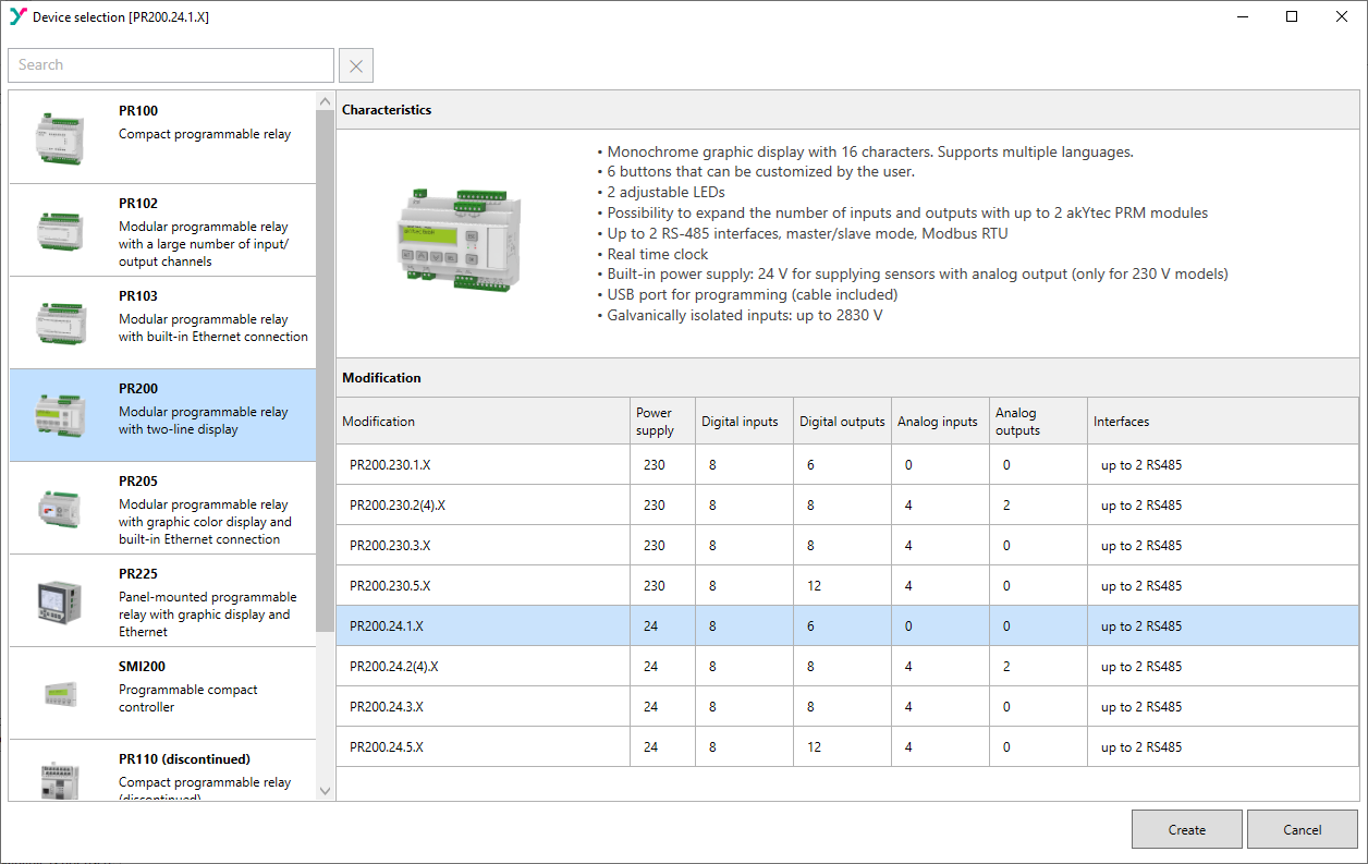
Figure 1: The available devices list, our selection for this course.
⚠️ Important Integrator Note: Hardware Selection & Output Constraints
As a professional engineering practitioner, you should never pick up a specific control module like the akYtec PR200 blindly just because a lesson focuses on it. True system design demands that you carefully study, evaluate, and choose your hardware architecture based entirely on your exact industrial use case requirements. While the underlying FBD logic program remains highly similar across different systems, where and how that logic interfaces with physical machinery changes everything before you click “buy.”
For instance, do your field elements require rapid, wear-free high-speed pulses, or do they switch heavy, inductive high-amperage loads? To fully master this core hardware engineering fork, check out our in-depth comparison guide: Transistor vs. Relay: Which Switch for Your Automation?
⚡ Crucial PR200 Electrical Architecture Alert: When analyzing this particular PR200 relay variant, take note of its input and output connection grouping constraints:
- The Input Split: The 8 digital inputs utilize two grouped common ground references (labeled COM1 and COM2). This architecture is perfectly safe and functional for the vast majority of sensor loops.
- The Output Shared Traps: The problem arises on the output side. The 6 digital outputs share only 3 common terminals. This means the mechanical relay contacts are not electrically independent from each other.
- The Electrical Consequence: If you inject a specific control voltage or a fast PWM signal into the first common terminal point (e.g., to run a 24V valve on Q1), output Q2 is completely forced to utilize that exact same electrical voltage supply source parameter. You cannot run a completely separate, isolated voltage loop channel on that paired block. Always map out your shared output potentials during your blueprint design stage to prevent catastrophic short circuits on your terminal blocks!
Click the New project icon or File ➔ New project (Ctrl+N). The development workspace environment will initialize instantly, loading a blank visual canvas framed by a blue bounding layout box. The interface populates terminal boxes mapped directly to physical components: inputs I1 to I8 on the upper side, while outputs Q1 to Q6 are situated on the bottom. You will also notice two specialized output markers labeled F1 and F2; these represent internal firmware functions rather than physical hardware relay contacts, and we will explore their usage later in the course.
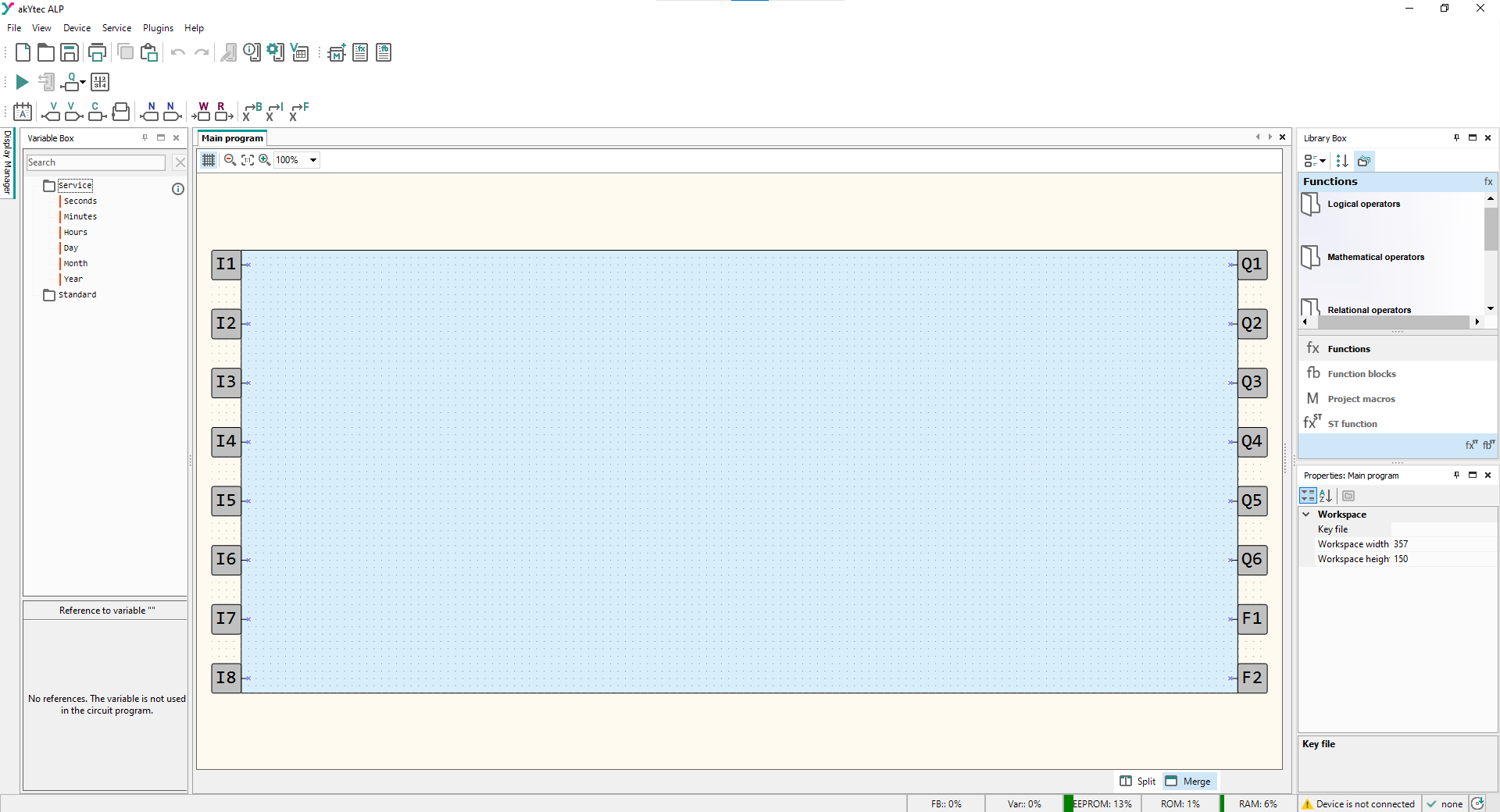
Figure 2: The initialized akYtec ALP canvas interface for an empty new PR200-24.1.X project.
🎨 Step 3: Navigating and Understanding the ALP Interface
The akYtec ALP development environment organizes its programming features into high-efficiency lateral docks. This layout maximizes your central design space while keeping hardware monitoring details fully visible.
- The Central Canvas: Framed by the blue system bounding box, this is your primary visual development environment where you arrange logic modules, drop function blocks, and map wire pathways.
- The Left Navigation Dock: This workspace area houses the Variables Box for defining local, network, and physical memory parameters, alongside the Display Manager dock. The Display Manager acts as your gateway to organizing screen navigation trees and customizing text fields for the onboard physical LCD screen.
- The Right Tool Pane: Divided into three distinct vertical zones for precise block management:
- The Middle Section (Core Selection): Your core components index directory. This is where you toggle major design types like “Functions”, “Function Blocks”, or custom macros.
- The Top Section (Visual Element Viewer): Serves as a dynamic viewer context screen for the middle panel. When you highlight an element category like “Functions” in the middle, this top block instantly expands to display all specific, available programming gates and operational logic nodes matching your selection.
- The Bottom Section (Properties & Scope): Houses the properties editor, allowing you to configure object parameters (like timer preset values) and redefine your core workspace grid canvas dimensions.
- The Top Toolbar: Hosts file operations, zoom utilities, layout alignments, and compilation controls. We will explore these specific operational tools as we deploy them across upcoming design steps, but you can always cross-reference the official software reference manual for comprehensive button-by-button breakdowns.
- The Bottom-Right Status Bar: Serves as your real-time hardware diagnostics link, continuously reporting hardware communication port configurations, internal device status, firmware memory allocation overhead metrics, and active connection layers.
🚀 Step 4: Building the “Hello World” Latching Logic
In the industrial automation sector, a “Hello World” application is not about printing a line of text to a console screen. Instead, it is about latching a mechanical relay safely. We will configure a dedicated RS Flip-Flop circuit where one digital button sets our output active, and a completely separate button resets it back to zero.
- Locating the Function Block: Navigate to the right-side tool pane. In the middle section (Core Selection), locate the option labeled Function Blocks—identifiable by the distinctive “fb” lettering icon—and click it once.
- Placing the RS Trigger: The right-side top section (Visual Element Viewer) will instantly populate with categories. Double-click the Triggers folder group, select the RS block from the checklist, and drag-and-drop it directly onto the open canvas workspace inside the blue project container box.
- Wiring Input I1 (The Set Trigger): Move your mouse cursor over to the left side of the blue canvas boundary box where your physical inputs are lined up. Locate the output node on the right edge of input I1, which is marked by a small “x” indicator. Hovering your mouse directly over this point transforms your cursor arrow into a dedicated wiring crosshair tool.
- Drawing the Path: Left-click once directly over the “x” node of I1 (do not hold the mouse button down). Drag your mouse path smoothly toward the center canvas area until you meet the top S (Set) input terminal node of your newly placed RS1 block, then left-click a second time to snap the wire track securely in place.
- Wiring Input I2 (The Reset Trigger): Repeat this click-and-snap technique to route a new connection pathway. Run a wire from the “x” terminal node of physical input I2 straight over into the lower R (Reset) input terminal pin of the RS1 trigger block.
- Wiring the Physical Output (Q1): To complete the visual program routing loop, click once over the output node labeled Q on the right-hand edge of your RS1 flip-flop block. Pull your wiring line across the canvas grid and click straight onto the physical terminal connection box labeled Q1 on the right boundary border.
💡 Pro UI Readability Habit (Wire Routing Optimization): As your visual function block sheets grow, crossing multiple raw wire tracks can become confusing. To maintain clean, professional readability, left-click directly over any active wire line you want to organize. The editor will expose a series of bright green adjustment handles. Simply click and drag these green dots to cleanly route your wire layouts away from other block headers, ensuring your pathways never cover or obscure each other.
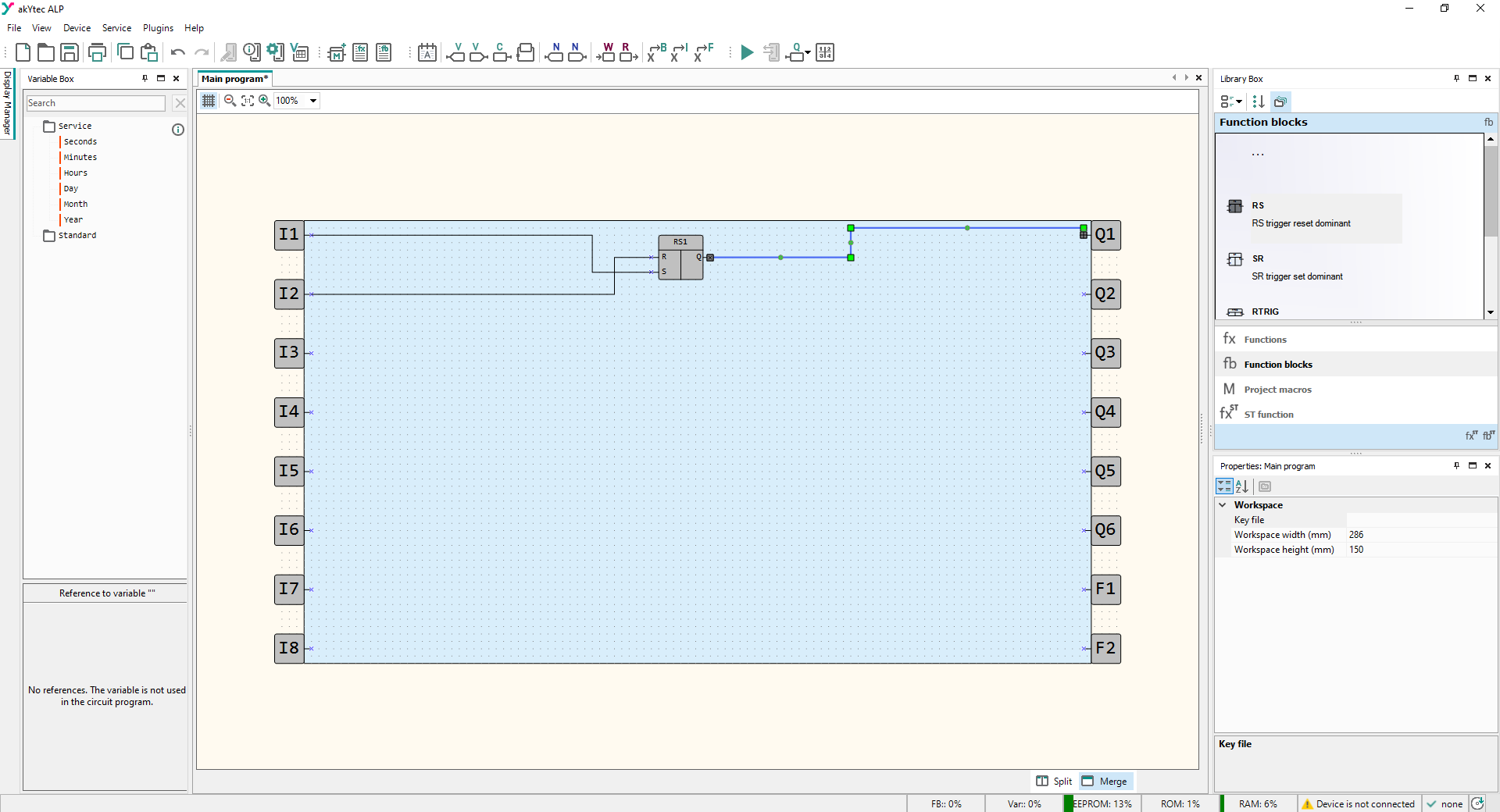
Figure 3: The RS function block cleanly connected and routed to the physical I/O terminals.
🧪 Step 5: Master Offline Emulation & the Watch Window Diagnostics
You do not need a physical PR200 unit on your bench to fully validate your automation logic. The akYtec ALP software framework features a built-in, real-time logic simulation engine that lets you safely map, force, and debug your data paths in software.
- Toolbar Realignment Pro-Tip: Before initiating the test, notice that you can manually rearrange the toolbars at the top of your interface window. Dragging them into a single horizontal row frees up maximum pixel space for your central canvas workspace. By default, these toolbars stack vertically organized into different categories, which can compress your design field.
- Activating the Simulator: Click the global Simulation Icon (the green triangle button) located in the upper toolbar array, or use the quick keyboard shortcut Shift + F5.
- The Intermediary State Buffer: Once activated, your entire project canvas layout shifts to a muted grey color, and all logic components and wire lines lock safely into a read-only configuration. The software drops into a strategic intermediary simulation state rather than executing the logic loops immediately. This pause is vital because it lets you pre-configure your initial physical hardware inputs (high, low, or sensor default states) before processing any live automation routines.
- The Simulation Tools Profile: A new specialized runtime toolbar will generate across your menu dock. This pane features timebase configuration fields (Cycle time and Refresh time), standard media player execution keys, and an advanced Watch Window module designed to trace live system data points sequentially.
- Configuring Your Watch Window: Move your mouse cursor over onto the physical Q1 output box on the right edge of your canvas. Right-click directly over the component block and select the single pop-up option labeled “Add to Watch Window”.
- Analyzing the Diagnostics Array: Look down at the bottom of your screen container area. The Watch Window has populated a structured data logging row for your selected output channel. It displays the variable name, its raw runtime value (currently showing a baseline string of “0”), and its data parameter type (labeled as a BOOL expression, which represents binary states of 0 or 1). For this entry-level evaluation run, leave your cycle and refresh configuration rates at their native system defaults.
- Firing Up Engine Execution: Click the second inline Green Start Button inside your fresh simulator toolbar array, or use the keyboard shortcut F6. The start button will turn grey to confirm that live logic processing loop routines are actively scanning your sheets.
- Understanding Runtime Flow Controls: While the simulator engine is actively scanning, your navigation toolbar presents three distinct operation choices:
- Pressing the “||” (Pause) button stops code iteration instantly while preserving your current runtime memory values.
- Pressing the Red Square (Stop) button completely resets your running logic execution loops back to zero.
- Pressing the original Simulation Icon (Green Triangle) terminates the emulation cycle entirely, closing your test windows and returning you safely back to standard canvas block editing mode.
🕹️ Executing the Latching Sequence Verification Test
With execution loops actively scanning, notice that every single logic node and terminal box on your canvas workspace displays its current numerical value depending on its data type. Because the network is completely at rest, your inputs and outputs display a standard baseline value string of 0.
- Simulate the START Pulse: Left-click once directly on the physical input box labeled I1 on the left side of your canvas. This forces the digital channel from a 0 to a 1 state. Left-click the I1 box a second time to drop it back to 0. This dual-click sequence perfectly mirrors pressing and releasing a real-world physical momentary start push-button on a machine panel.
- Observe the Latch Response: Look closely at your canvas layout and down at your diagnostics dashboard. The RS1 flip-flop block catches that temporary pulse and instantly locks its output high. In your active Watch Window, the variable row for Q1 updates to read 1. Simultaneously, the physical output box container for Q1 on your canvas template turns bright red (signaling a live HIGH state), and its inline numerical display flips from 0 to 1. Even though your start input I1 fell completely back to 0, the internal logic holds the state perfectly—this is industrial automation memory in action!
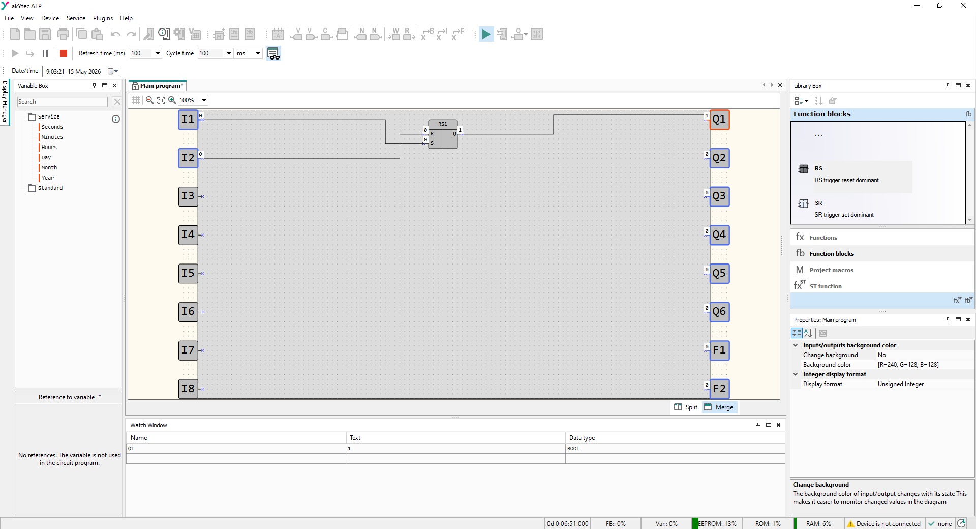
Figure 4: The RS latching logic circuit operating in live simulation mode with the Q1 output driven high (red path).
- Simulate the STOP Pulse: To break the loop latch and turn the output off, left-click twice on your I2 input terminal box to send a clean momentary stop pulse. The RS1 block registers the signal on its Reset pin, drops its internal latch, turns the physical output terminal box back to grey, and drops your Watch Window registry value cleanly back down to 0.
🎉 Congratulations, Industrial Integrator! You have successfully finished akYtec ALP Lesson 1. You have moved your workstation environment over into a professional visual development architecture, structured a resilient dual-point latching system based entirely on real hardware parameters, and verified execution using advanced runtime debugging windows.
Ready to Bring Your Logic to Life?
You have successfully structured your visual latching code and fully validated its paths in simulation. Now, it’s time to bridge software design with actual factory-floor physics.